Tutorial: optimal binning 2D with continuous target
To get us started, let’s load a well-known dataset from the UCI repository and transform the data into a pandas.DataFrame.
[1]:
import numpy as np
import pandas as pd
[2]:
class Data:
    def __init__(self, data, target, feature_names):
        self.data = data
        self.target = target
        self.feature_names = feature_names


def load_boston():
    data_url = "../../../tests/data/boston_housing.csv"
    raw_df = pd.read_csv(data_url, sep=r"\s+", skiprows=22, header=None)
    raw_data = np.hstack([raw_df.values[::2, :], raw_df.values[1::2, :2]])
    target = raw_df.values[1::2, 2]
    feature_names = ['CRIM', 'ZN', 'INDUS', 'CHAS', 'NOX', 'RM', 'AGE', 'DIS',
                     'RAD', 'TAX', 'PTRATIO', 'B', 'LSTAT']

    return Data(raw_data, target, feature_names)


data = load_boston()
df = pd.DataFrame(data.data, columns=data.feature_names)
We choose two variables to discretize and the continuous target.
[3]:
variable1 = "AGE"
variable2 = "INDUS"

x = df[variable1].values
y = df[variable2].values
z = data.target
Import and instantiate an ContinuousOptimalBinning2D object class. We pass the variable names (coordinates x and y), and a solver, in this case, we choose the constraint programming solver.
[4]:
from optbinning import ContinuousOptimalBinning2D
[5]:
optb = ContinuousOptimalBinning2D(name_x=variable1, name_y=variable2, solver="cp")
We fit the optimal binning object with arrays x, y, and z.
[6]:
optb.fit(x, y, z)
[6]:
ContinuousOptimalBinning2D(name_x='AGE', name_y='INDUS')In a Jupyter environment, please rerun this cell to show the HTML representation or trust the notebook.
On GitHub, the HTML representation is unable to render, please try loading this page with nbviewer.org.
Parameters
| name_x | 'AGE' | |
| name_y | 'INDUS' | |
| dtype_x | 'numerical' | |
| dtype_y | 'numerical' | |
| prebinning_method | 'cart' | |
| strategy | 'grid' | |
| solver | 'cp' | |
| max_n_prebins_x | 5 | |
| max_n_prebins_y | 5 | |
| min_prebin_size_x | 0.05 | |
| min_prebin_size_y | 0.05 | |
| min_n_bins | None | |
| max_n_bins | None | |
| min_bin_size | None | |
| max_bin_size | None | |
| monotonic_trend_x | None | |
| monotonic_trend_y | None | |
| min_mean_diff_x | 0 | |
| min_mean_diff_y | 0 | |
| gamma | 0 | |
| special_codes_x | None | |
| special_codes_y | None | |
| split_digits | None | |
| n_jobs | 1 | |
| time_limit | 100 | |
| verbose | False |
Similar to other OptBinning classes, you can inspect the attributes status and splits. In this case, the splits shown are actually the bins, but the splits name is used to maintain API homogeneity.
[7]:
optb.status
[7]:
'OPTIMAL'
[8]:
optb.splits
[8]:
([[np.float64(-inf), np.float64(37.25)],
  [np.float64(37.25), np.float64(76.25)],
  [np.float64(76.25), np.float64(92.29999923706055)],
  [np.float64(92.29999923706055), np.float64(98.25)],
  [np.float64(98.25), np.float64(inf)],
  [np.float64(-inf), np.float64(37.25)],
  [np.float64(37.25), np.float64(76.25)],
  [np.float64(76.25), np.float64(92.29999923706055)],
  [np.float64(92.29999923706055), np.float64(98.25)],
  [np.float64(-inf), np.float64(37.25)],
  [np.float64(37.25), np.float64(76.25)],
  [np.float64(76.25), np.float64(92.29999923706055)],
  [np.float64(92.29999923706055), np.float64(98.25)],
  [np.float64(98.25), np.float64(inf)],
  [np.float64(-inf), np.float64(37.25)],
  [np.float64(37.25), np.float64(76.25)],
  [np.float64(76.25), np.float64(92.29999923706055)],
  [np.float64(37.25), np.float64(76.25)],
  [np.float64(76.25), np.float64(92.29999923706055)],
  [np.float64(92.29999923706055), np.float64(98.25)],
  [np.float64(98.25), np.float64(inf)]],
 [[np.float64(-inf), np.float64(3.9850000143051147)],
  [np.float64(-inf), np.float64(3.9850000143051147)],
  [np.float64(-inf), np.float64(3.9850000143051147)],
  [np.float64(-inf), np.float64(3.9850000143051147)],
  [np.float64(-inf), np.float64(6.080000162124634)],
  [np.float64(3.9850000143051147), np.float64(6.080000162124634)],
  [np.float64(3.9850000143051147), np.float64(6.080000162124634)],
  [np.float64(3.9850000143051147), np.float64(6.080000162124634)],
  [np.float64(3.9850000143051147), np.float64(6.080000162124634)],
  [np.float64(6.080000162124634), np.float64(6.659999847412109)],
  [np.float64(6.080000162124634), np.float64(6.659999847412109)],
  [np.float64(6.080000162124634), np.float64(6.659999847412109)],
  [np.float64(6.080000162124634), np.float64(16.570000171661377)],
  [np.float64(6.080000162124634), np.float64(16.570000171661377)],
  [np.float64(6.659999847412109), np.float64(inf)],
  [np.float64(6.659999847412109), np.float64(16.570000171661377)],
  [np.float64(6.659999847412109), np.float64(16.570000171661377)],
  [np.float64(16.570000171661377), np.float64(inf)],
  [np.float64(16.570000171661377), np.float64(inf)],
  [np.float64(16.570000171661377), np.float64(inf)],
  [np.float64(16.570000171661377), np.float64(inf)]])
The binning table
The binning table follows the same structure as the unidimensional binning, except for having two Bin columns, one for each variable (coordinate). The option show_bin_xy=True in method build combines both columns to obtain a single Bin column.
[9]:
optb.binning_table.build()
[9]:
| Bin x | Bin y | Count | Count (%) | Sum | Std | Mean | WoE | IV | |
|---|---|---|---|---|---|---|---|---|---|
| 0 | (-inf, 37.25) | (-inf, 3.99) | 43 | 0.084980 | 1317.3 | 9.113544 | 30.634884 | 8.102077 | 0.688516 |
| 1 | [37.25, 76.25) | (-inf, 3.99) | 35 | 0.069170 | 1115.1 | 8.144242 | 31.860000 | 9.327194 | 0.645162 |
| 2 | [76.25, 92.30) | (-inf, 3.99) | 10 | 0.019763 | 370.6 | 8.343644 | 37.060000 | 14.527194 | 0.287099 |
| 3 | [92.30, 98.25) | (-inf, 3.99) | 2 | 0.003953 | 63.5 | 0.75 | 31.750000 | 9.217194 | 0.036432 |
| 4 | [98.25, inf) | (-inf, 6.08) | 2 | 0.003953 | 66.1 | 2.95 | 33.050000 | 10.517194 | 0.041570 |
| 5 | (-inf, 37.25) | [3.99, 6.08) | 27 | 0.053360 | 680.8 | 5.262706 | 25.214815 | 2.682008 | 0.143111 |
| 6 | [37.25, 76.25) | [3.99, 6.08) | 36 | 0.071146 | 773.6 | 2.676002 | 21.488889 | -1.043917 | 0.074271 |
| 7 | [76.25, 92.30) | [3.99, 6.08) | 4 | 0.007905 | 84.8 | 2.388514 | 21.200000 | -1.332806 | 0.010536 |
| 8 | [92.30, 98.25) | [3.99, 6.08) | 1 | 0.001976 | 16.0 | 0.0 | 16.000000 | -6.532806 | 0.012911 |
| 9 | (-inf, 37.25) | [6.08, 6.66) | 7 | 0.013834 | 232.3 | 5.962365 | 33.185714 | 10.652908 | 0.147372 |
| 10 | [37.25, 76.25) | [6.08, 6.66) | 9 | 0.017787 | 286.0 | 8.119357 | 31.777778 | 9.244971 | 0.164436 |
| 11 | [76.25, 92.30) | [6.08, 6.66) | 10 | 0.019763 | 326.8 | 8.488086 | 32.680000 | 10.147194 | 0.200537 |
| 12 | [92.30, 98.25) | [6.08, 16.57) | 15 | 0.029644 | 264.7 | 4.036478 | 17.646667 | -4.886140 | 0.144846 |
| 13 | [98.25, inf) | [6.08, 16.57) | 4 | 0.007905 | 65.5 | 2.246525 | 16.375000 | -6.157806 | 0.048678 |
| 14 | (-inf, 37.25) | [6.66, inf) | 23 | 0.045455 | 543.5 | 2.32761 | 23.630435 | 1.097628 | 0.049892 |
| 15 | [37.25, 76.25) | [6.66, 16.57) | 49 | 0.096838 | 1086.8 | 3.434815 | 22.179592 | -0.353214 | 0.034205 |
| 16 | [76.25, 92.30) | [6.66, 16.57) | 40 | 0.079051 | 777.0 | 3.359967 | 19.425000 | -3.107806 | 0.245676 |
| 17 | [37.25, 76.25) | [16.57, inf) | 16 | 0.031621 | 324.4 | 4.472765 | 20.275000 | -2.257806 | 0.071393 |
| 18 | [76.25, 92.30) | [16.57, inf) | 50 | 0.098814 | 912.5 | 8.416228 | 18.250000 | -4.282806 | 0.423202 |
| 19 | [92.30, 98.25) | [16.57, inf) | 71 | 0.140316 | 1286.2 | 10.093278 | 18.115493 | -4.417313 | 0.619821 |
| 20 | [98.25, inf) | [16.57, inf) | 52 | 0.102767 | 808.1 | 8.66228 | 15.540385 | -6.992422 | 0.718589 |
| 21 | Special | Special | 0 | 0.000000 | 0.0 | 0.0 | 0.000000 | -22.532806 | 0.000000 |
| 22 | Missing | Missing | 0 | 0.000000 | 0.0 | 0.0 | 0.000000 | -22.532806 | 0.000000 |
| Totals | 506 | 1.000000 | 11401.6 | 22.532806 | 171.946019 | 4.808255 |
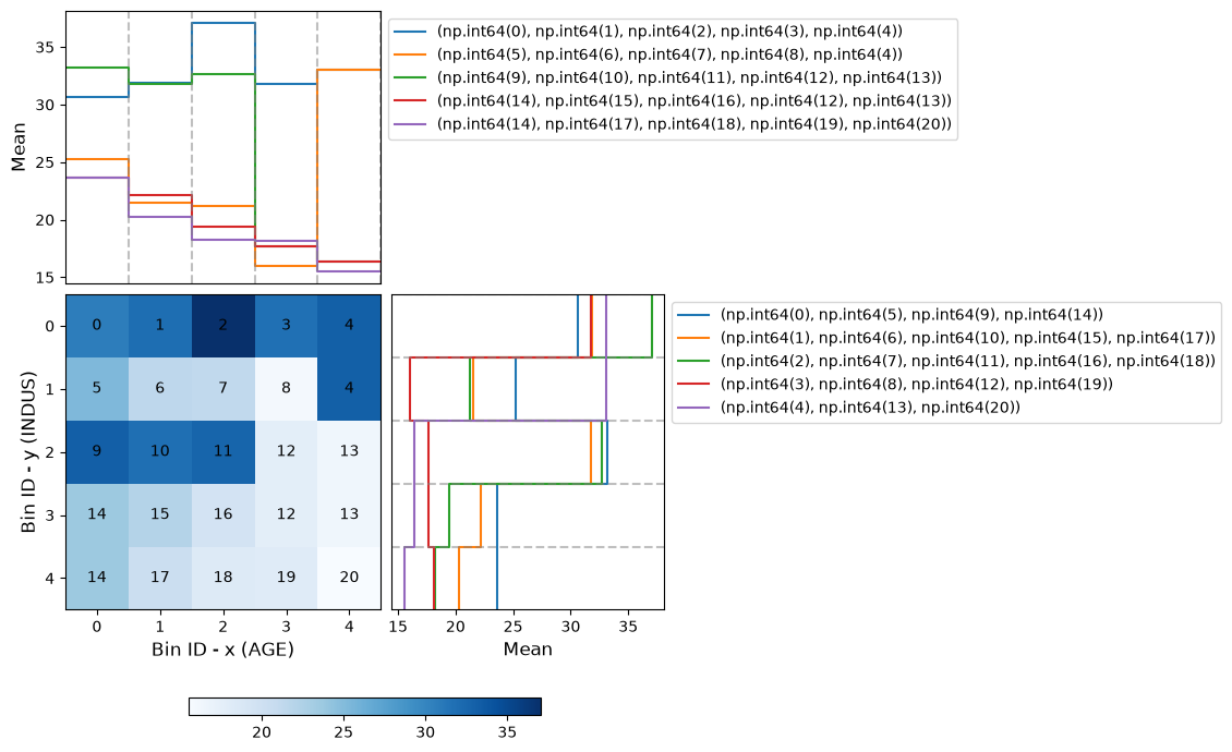
You can use the method plot to visualize the histogram 2D and mean curve. Note that the Bin ID corresponds to the binning table index. These are the key points to correctly interpret the plots belows:
Bins can only be rectangles. If a bin is composed by \(m\) squares, the Bin ID is shown \(m\) times.
The upper left plot shows the mean on the x-axis; the bin paths left-right.
The lower right plot shows the mean on the y-axis; the bin paths top-down.
[10]:
optb.binning_table.plot()
Mean transformation
Now that we have checked the binned data, we can transform our original data into mean values. You can check the correctness of the transformation using pandas value_counts method, for instance. Note that both x and y are required, and a single array is returned with the transformation.
[11]:
z_transform_mean = optb.transform(x, y, metric="mean")
pd.Series(z_transform_mean).value_counts()
[11]:
18.115493    71
15.540385    52
18.250000    50
22.179592    49
30.634884    43
19.425000    40
21.488889    36
31.860000    35
25.214815    27
23.630435    23
20.275000    16
17.646667    15
37.060000    10
32.680000    10
31.777778     9
33.185714     7
16.375000     4
21.200000     4
31.750000     2
33.050000     2
16.000000     1
Name: count, dtype: int64
[12]:
z_transform_indices = optb.transform(x, y, metric="indices")
pd.Series(z_transform_indices).value_counts()
[12]:
19    71
20    52
18    50
15    49
0     43
16    40
6     36
1     35
5     27
14    23
17    16
12    15
2     10
11    10
10     9
9      7
13     4
7      4
3      2
4      2
8      1
Name: count, dtype: int64
If metric="bins" the bin ids are combined.
[13]:
z_transform_bins = optb.transform(x, y, metric="bins")
pd.Series(z_transform_bins).value_counts()
[13]:
[92.30, 98.25) $\cup$ [16.57, inf)     71
[98.25, inf) $\cup$ [16.57, inf)       52
[76.25, 92.30) $\cup$ [16.57, inf)     50
[37.25, 76.25) $\cup$ [6.66, 16.57)    49
(-inf, 37.25) $\cup$ (-inf, 3.99)      43
[76.25, 92.30) $\cup$ [6.66, 16.57)    40
[37.25, 76.25) $\cup$ [3.99, 6.08)     36
[37.25, 76.25) $\cup$ (-inf, 3.99)     35
(-inf, 37.25) $\cup$ [3.99, 6.08)      27
(-inf, 37.25) $\cup$ [6.66, inf)       23
[37.25, 76.25) $\cup$ [16.57, inf)     16
[92.30, 98.25) $\cup$ [6.08, 16.57)    15
[76.25, 92.30) $\cup$ (-inf, 3.99)     10
[76.25, 92.30) $\cup$ [6.08, 6.66)     10
[37.25, 76.25) $\cup$ [6.08, 6.66)      9
(-inf, 37.25) $\cup$ [6.08, 6.66)       7
[98.25, inf) $\cup$ [6.08, 16.57)       4
[76.25, 92.30) $\cup$ [3.99, 6.08)      4
[92.30, 98.25) $\cup$ (-inf, 3.99)      2
[98.25, inf) $\cup$ (-inf, 6.08)        2
[92.30, 98.25) $\cup$ [3.99, 6.08)      1
Name: count, dtype: int64
Binning table statistical analysis
The analysis method performs a statistical analysis of the binning table, computing the Information Value (IV), Weight of Evidence (WoE), and Herfindahl-Hirschman Index (HHI). The report is the same that the one for unidimensional binning with a continuous target. The main difference is that the significant tests for each bin are performed with respect to all its linked bins.
[14]:
optb.binning_table.analysis()
----------------------------------------------------
OptimalBinning: Continuous Binning Table 2D Analysis
----------------------------------------------------

  General metrics

    IV                       4.80825509
    WoE                    171.94601939
    WoE (normalized)         7.63091898
    HHI                      0.08094955
    HHI (normalized)         0.03499703
    Quality score            0.00000048

  Significance tests

    Bin A  Bin B  t-statistic      p-value
        0      1    -0.626279 5.330261e-01
        0      5     3.151772 2.418667e-03
        1      2    -1.747295 1.020375e-01
        1      6     7.166955 9.494930e-09
        2      3     1.973052 7.794888e-02
        2      7     5.476169 1.595659e-04
        3      4    -0.603998 6.445191e-01
        3      8    29.698485 2.142801e-02
        4     13     7.038328 3.332810e-02
        5      6     3.366820 1.818855e-03
        5      9    -3.226180 1.104060e-02
        6      7     0.226611 8.321374e-01
        6     10    -3.751024 5.101241e-03
        7      8     4.354171 1.437169e-01
        7     11    -3.907609 2.230164e-03
        8      4    -8.173675 7.750145e-02
        8     12    -1.579970 3.592298e-01
        9     10     0.399772 6.953661e-01
        9     14     4.145039 4.969267e-03
       10     11    -0.236693 8.157359e-01
       10     15     3.489521 7.419876e-03
       11     12     5.220987 2.298907e-04
       11     16     4.844244 7.355489e-04
       12     13     0.829910 4.281352e-01
       12     19    -0.295271 7.688809e-01
       13     20     0.507489 6.204418e-01
       14     15     2.102164 3.968648e-02
       14     17     2.752663 1.203338e-02
       15     16     3.808928 2.644745e-04
       15     17     1.559713 1.337095e-01
       16     12     1.520196 1.429031e-01
       16     18     0.901478 3.705578e-01
       17     18     1.239974 2.208911e-01
       18     19     0.079654 9.366502e-01
       19     20     1.517969 1.316990e-01
Mean monotonicity
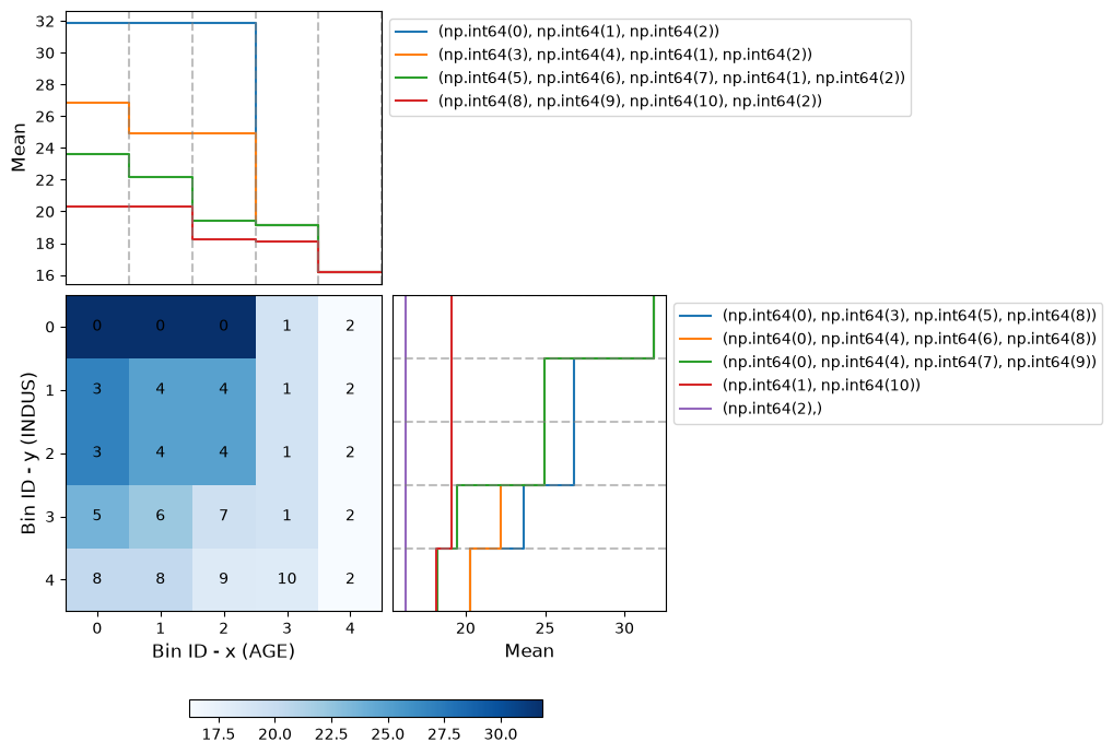
The monotonic_trend_x and monotonic_trend_y options permit forcing a monotonic trend to the mean curve on each axis. By default, both options are set to None. There are two options available: “ascending” and “descending”. In this example, we force both trends to be “descending”, and a minimum bin size of 0.025 (2.5%).
[15]:
optb = ContinuousOptimalBinning2D(name_x=variable1, name_y=variable2,
                                  monotonic_trend_x="descending",
                                  monotonic_trend_y="descending", min_bin_size=0.025)
optb.fit(x, y, z)
[15]:
ContinuousOptimalBinning2D(min_bin_size=0.025, monotonic_trend_x='descending',
                           monotonic_trend_y='descending', name_x='AGE',
                           name_y='INDUS')
In a Jupyter environment, please rerun this cell to show the HTML representation or trust the notebook. On GitHub, the HTML representation is unable to render, please try loading this page with nbviewer.org.
Parameters
| name_x | 'AGE' | |
| name_y | 'INDUS' | |
| min_bin_size | 0.025 | |
| monotonic_trend_x | 'descending' | |
| monotonic_trend_y | 'descending' | |
| dtype_x | 'numerical' | |
| dtype_y | 'numerical' | |
| prebinning_method | 'cart' | |
| strategy | 'grid' | |
| solver | 'cp' | |
| max_n_prebins_x | 5 | |
| max_n_prebins_y | 5 | |
| min_prebin_size_x | 0.05 | |
| min_prebin_size_y | 0.05 | |
| min_n_bins | None | |
| max_n_bins | None | |
| max_bin_size | None | |
| min_mean_diff_x | 0 | |
| min_mean_diff_y | 0 | |
| gamma | 0 | |
| special_codes_x | None | |
| special_codes_y | None | |
| split_digits | None | |
| n_jobs | 1 | |
| time_limit | 100 | |
| verbose | False |
[16]:
optb.binning_table.build()
[16]:
| Bin x | Bin y | Count | Count (%) | Sum | Std | Mean | WoE | IV | |
|---|---|---|---|---|---|---|---|---|---|
| 0 | (-inf, 92.30) | (-inf, 3.99) | 88 | 0.173913 | 2803.0 | 8.870303 | 31.852273 | 9.319466 | 1.620777 |
| 1 | [92.30, 98.25) | (-inf, 16.57) | 18 | 0.035573 | 344.2 | 5.806372 | 19.122222 | -3.410584 | 0.121325 |
| 2 | [98.25, inf) | (-inf, inf) | 58 | 0.114625 | 939.7 | 8.837625 | 16.201724 | -6.331082 | 0.725697 |
| 3 | (-inf, 37.25) | [3.99, 6.66) | 34 | 0.067194 | 913.1 | 6.300849 | 26.855882 | 4.323076 | 0.290483 |
| 4 | [37.25, 92.30) | [3.99, 6.66) | 59 | 0.116601 | 1471.2 | 7.247437 | 24.935593 | 2.402787 | 0.280167 |
| 5 | (-inf, 37.25) | [6.66, 16.57) | 23 | 0.045455 | 543.5 | 2.32761 | 23.630435 | 1.097628 | 0.049892 |
| 6 | [37.25, 76.25) | [6.66, 16.57) | 49 | 0.096838 | 1086.8 | 3.434815 | 22.179592 | -0.353214 | 0.034205 |
| 7 | [76.25, 92.30) | [6.66, 16.57) | 40 | 0.079051 | 777.0 | 3.359967 | 19.425000 | -3.107806 | 0.245676 |
| 8 | (-inf, 76.25) | [16.57, inf) | 16 | 0.031621 | 324.4 | 4.472765 | 20.275000 | -2.257806 | 0.071393 |
| 9 | [76.25, 92.30) | [16.57, inf) | 50 | 0.098814 | 912.5 | 8.416228 | 18.250000 | -4.282806 | 0.423202 |
| 10 | [92.30, 98.25) | [16.57, inf) | 71 | 0.140316 | 1286.2 | 10.093278 | 18.115493 | -4.417313 | 0.619821 |
| 11 | Special | Special | 0 | 0.000000 | 0.0 | 0.0 | 0.000000 | -22.532806 | 0.000000 |
| 12 | Missing | Missing | 0 | 0.000000 | 0.0 | 0.0 | 0.000000 | -22.532806 | 0.000000 |
| Totals | 506 | 1.000000 | 11401.6 | 22.532806 | 86.369184 | 4.482638 |
[17]:
optb.binning_table.plot()
[18]:
optb.binning_table.analysis()
----------------------------------------------------
OptimalBinning: Continuous Binning Table 2D Analysis
----------------------------------------------------

  General metrics

    IV                       4.48263838
    WoE                     86.36918355
    WoE (normalized)         3.83304158
    HHI                      0.11090628
    HHI (normalized)         0.02199691
    Quality score            0.00065845

  Significance tests

    Bin A  Bin B  t-statistic      p-value
        0      1     7.652734 5.085335e-09
        0      3     3.479643 7.978542e-04
        0      4     5.177909 7.689996e-07
        1      2     1.627628 1.108228e-01
        1     10     0.553529 5.825586e-01
        3      4     1.338602 1.846378e-01
        3      5     2.722868 9.181932e-03
        4      1     3.497175 1.308292e-03
        4      6     2.591442 1.122681e-02
        4      7     5.089123 2.035925e-06
        5      6     2.102164 3.968648e-02
        5      8     2.752663 1.203338e-02
        6      7     3.808928 2.644745e-04
        6      8     1.559713 1.337095e-01
        7      1     0.206242 8.384742e-01
        7      9     0.901478 3.705578e-01
        8      9     1.239974 2.208911e-01
        9     10     0.079654 9.366502e-01
       10      2     1.147500 2.533428e-01
Mininum mean difference between consecutive bins
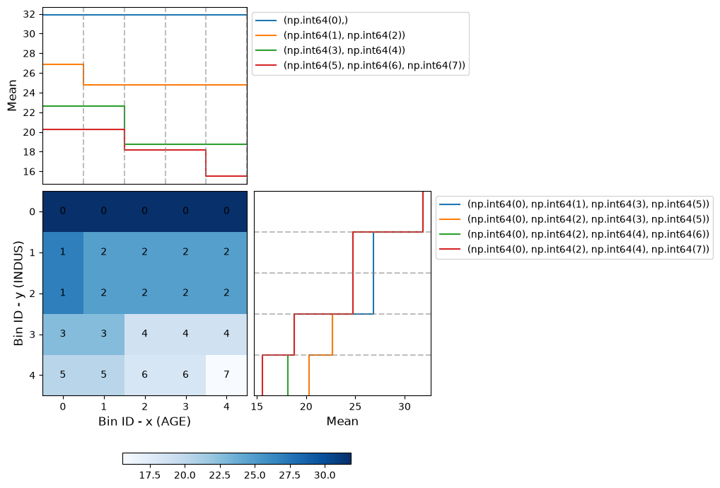
Now, we note that the mean difference between consecutive bins is not significant enough on the x-axis. Therefore, we decide to set min_mean_diff_x=2.0:
[19]:
optb = ContinuousOptimalBinning2D(name_x=variable1, name_y=variable2,
                                  monotonic_trend_x="descending",
                                  monotonic_trend_y="descending", min_bin_size=0.025,
                                  min_mean_diff_x=2.0)
optb.fit(x, y, z)
[19]:
ContinuousOptimalBinning2D(min_bin_size=0.025, min_mean_diff_x=2.0,
                           monotonic_trend_x='descending',
                           monotonic_trend_y='descending', name_x='AGE',
                           name_y='INDUS')
In a Jupyter environment, please rerun this cell to show the HTML representation or trust the notebook. On GitHub, the HTML representation is unable to render, please try loading this page with nbviewer.org.
Parameters
| name_x | 'AGE' | |
| name_y | 'INDUS' | |
| min_bin_size | 0.025 | |
| monotonic_trend_x | 'descending' | |
| monotonic_trend_y | 'descending' | |
| min_mean_diff_x | 2.0 | |
| dtype_x | 'numerical' | |
| dtype_y | 'numerical' | |
| prebinning_method | 'cart' | |
| strategy | 'grid' | |
| solver | 'cp' | |
| max_n_prebins_x | 5 | |
| max_n_prebins_y | 5 | |
| min_prebin_size_x | 0.05 | |
| min_prebin_size_y | 0.05 | |
| min_n_bins | None | |
| max_n_bins | None | |
| max_bin_size | None | |
| min_mean_diff_y | 0 | |
| gamma | 0 | |
| special_codes_x | None | |
| special_codes_y | None | |
| split_digits | None | |
| n_jobs | 1 | |
| time_limit | 100 | |
| verbose | False |
[20]:
optb.binning_table.build()
[20]:
| Bin x | Bin y | Count | Count (%) | Sum | Std | Mean | WoE | IV | |
|---|---|---|---|---|---|---|---|---|---|
| 0 | (-inf, inf) | (-inf, 3.99) | 92 | 0.181818 | 2932.6 | 8.688703 | 31.876087 | 9.343281 | 1.698778 |
| 1 | (-inf, 37.25) | [3.99, 6.66) | 34 | 0.067194 | 913.1 | 6.300849 | 26.855882 | 4.323076 | 0.290483 |
| 2 | [37.25, inf) | [3.99, 6.66) | 60 | 0.118577 | 1487.2 | 7.277258 | 24.786667 | 2.253860 | 0.267256 |
| 3 | (-inf, 76.25) | [6.66, 16.57) | 72 | 0.142292 | 1630.3 | 3.196475 | 22.643056 | 0.110249 | 0.015688 |
| 4 | [76.25, inf) | [6.66, 16.57) | 59 | 0.116601 | 1107.2 | 3.624755 | 18.766102 | -3.766705 | 0.439201 |
| 5 | (-inf, 76.25) | [16.57, inf) | 16 | 0.031621 | 324.4 | 4.472765 | 20.275000 | -2.257806 | 0.071393 |
| 6 | [76.25, 98.25) | [16.57, inf) | 121 | 0.239130 | 2198.7 | 9.436718 | 18.171074 | -4.361732 | 1.043023 |
| 7 | [98.25, inf) | [16.57, inf) | 52 | 0.102767 | 808.1 | 8.66228 | 15.540385 | -6.992422 | 0.718589 |
| 8 | Special | Special | 0 | 0.000000 | 0.0 | 0.0 | 0.000000 | -22.532806 | 0.000000 |
| 9 | Missing | Missing | 0 | 0.000000 | 0.0 | 0.0 | 0.000000 | -22.532806 | 0.000000 |
| Totals | 506 | 1.000000 | 11401.6 | 22.532806 | 78.474743 | 4.544411 |
[21]:
optb.binning_table.plot()
[22]:
optb.binning_table.analysis()
----------------------------------------------------
OptimalBinning: Continuous Binning Table 2D Analysis
----------------------------------------------------

  General metrics

    IV                       4.54441094
    WoE                     78.47474349
    WoE (normalized)         3.48268841
    HHI                      0.15422050
    HHI (normalized)         0.03339486
    Quality score            0.18716085

  Significance tests

    Bin A  Bin B  t-statistic      p-value
        0      1     3.560295 6.228004e-04
        0      2     5.432189 2.380140e-07
        1      2     1.445094 1.524836e-01
        1      3     3.681359 6.667794e-04
        2      3     2.117773 3.738699e-02
        2      4     5.726516 1.440551e-07
        3      4     6.420686 3.039622e-09
        3      5     2.006927 5.955795e-02
        4      6     0.607723 5.441768e-01
        4      7     2.499373 1.491463e-02
        5      6     1.492816 1.441306e-01
        6      7     1.782159 7.762179e-02