Tutorial: optimal binning with binary target - large scale
Continuing with the previous tutorial, version 0.4.0 introduced four new monotonic_trend options: “auto_heuristic”, “auto_asc_desc”, “peak_heuristic” and “valley_heuristic”. These new heuristic options are devised to produce a remarkable speedup for large size instances, at the expense of not guaranteeing optimal solutions (although the optimal solution is found in the majority of cases).
Let’s start by loading the training data.
[1]:
import pandas as pd
[2]:
df = pd.read_csv("data/kaggle/HomeCreditDefaultRisk/application_train.csv", engine='c')
We choose the same variable to discretize and the binary target.
[3]:
variable = "REGION_POPULATION_RELATIVE"
x = df[variable].values
y = df.TARGET.values
[4]:
from optbinning import OptimalBinning
We use the same options to generate a granular binning, and fit the optimal binning with monotonic_trend="auto".
[5]:
optb = OptimalBinning(name=variable, dtype="numerical", solver="cp",
                      monotonic_trend="auto", max_n_prebins=100,
                      min_prebin_size=0.001, time_limit=200)
[6]:
optb.fit(x, y)
[6]:
OptimalBinning(max_n_prebins=100, min_prebin_size=0.001,
               name='REGION_POPULATION_RELATIVE', time_limit=200)
In a Jupyter environment, please rerun this cell to show the HTML representation or trust the notebook. On GitHub, the HTML representation is unable to render, please try loading this page with nbviewer.org.
Parameters
| name | 'REGION_POPULATION_RELATIVE' | |
| max_n_prebins | 100 | |
| min_prebin_size | 0.001 | |
| time_limit | 200 | |
| dtype | 'numerical' | |
| prebinning_method | 'cart' | |
| solver | 'cp' | |
| divergence | 'iv' | |
| min_n_bins | None | |
| max_n_bins | None | |
| min_bin_size | None | |
| max_bin_size | None | |
| min_bin_n_nonevent | None | |
| max_bin_n_nonevent | None | |
| min_bin_n_event | None | |
| max_bin_n_event | None | |
| monotonic_trend | 'auto' | |
| min_event_rate_diff | 0 | |
| max_pvalue | None | |
| max_pvalue_policy | 'consecutive' | |
| gamma | 0 | |
| outlier_detector | None | |
| outlier_params | None | |
| class_weight | None | |
| cat_cutoff | None | |
| cat_unknown | None | |
| user_splits | None | |
| user_splits_fixed | None | |
| special_codes | None | |
| split_digits | None | |
| mip_solver | 'bop' | |
| verbose | False |
[7]:
optb.status
[7]:
'FEASIBLE'
[8]:
optb.information(print_level=1)
optbinning (Version 1.0.0)
Copyright (c) 2019-2026 Guillermo Navas-Palencia, Apache License 2.0

  Name    : REGION_POPULATION_RELATIVE
  Status  : FEASIBLE

  Pre-binning statistics
    Number of pre-bins                    77
    Number of refinements                  0

  Solver statistics
    Type                                  cp
    Number of booleans                  3231
    Number of branches                 34159
    Number of conflicts                  623
    Objective value                    34366
    Best objective bound               74226

  Timing
    Total time                        207.83 sec
    Pre-processing                      0.01 sec   (  0.01%)
    Pre-binning                         0.54 sec   (  0.26%)
    Solver                            207.27 sec   ( 99.73%)
      model generation                  7.21 sec   (  3.48%)
      optimizer                       200.07 sec   ( 96.52%)
    Post-processing                     0.00 sec   (  0.00%)
[9]:
binning_table = optb.binning_table
binning_table.build()
binning_table.analysis()
---------------------------------------------
OptimalBinning: Binary Binning Table Analysis
---------------------------------------------

  General metrics

    Gini index               0.07378990
    IV (Jeffrey)             0.03437036
    JS (Jensen-Shannon)      0.00423897
    Hellinger                0.00426730
    Triangular               0.01673702
    KS                       0.06036678
    HHI                      0.27868030
    HHI (normalized)         0.19853367
    Cramer's V               0.04738095
    Quality score            0.00525816

  Monotonic trend                  peak

  Significance tests

    Bin A  Bin B  t-statistic      p-value  P[A > B]     P[B > A]
        0      1     8.076140 4.485187e-03  0.001401 9.985988e-01
        1      2    15.491601 8.287266e-05  0.000014 9.999860e-01
        2      3    68.103648 1.551234e-16  1.000000 4.019007e-14
        3      4     0.064167 8.000273e-01  0.601633 3.983667e-01
        4      5     0.086441 7.687514e-01  0.615314 3.846857e-01
        5      6    24.335649 8.092740e-07  1.000000 1.062350e-07
        6      7    40.662233 1.809509e-10  1.000000 1.110223e-16
        7      8    29.296187 6.211781e-08  1.000000 4.795253e-11
        8      9    10.992632 9.147483e-04  0.999765 2.351244e-04
[10]:
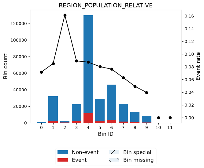
binning_table.plot(metric="event_rate")
This is a large combinatorial problem, and it took roughly 200 seconds to obtain a feasible solution… but we can try the monotonic_trend="auto_heuristic" to accelerate the solution process
[11]:
optb_auto = OptimalBinning(name=variable, dtype="numerical", solver="cp",
                           monotonic_trend="auto_heuristic", max_n_prebins=100,
                           min_prebin_size=0.001, time_limit=200)
[12]:
optb_auto.fit(x, y)
[12]:
OptimalBinning(max_n_prebins=100, min_prebin_size=0.001,
               monotonic_trend='auto_heuristic',
               name='REGION_POPULATION_RELATIVE', time_limit=200)
In a Jupyter environment, please rerun this cell to show the HTML representation or trust the notebook. On GitHub, the HTML representation is unable to render, please try loading this page with nbviewer.org.
Parameters
| name | 'REGION_POPULATION_RELATIVE' | |
| max_n_prebins | 100 | |
| min_prebin_size | 0.001 | |
| monotonic_trend | 'auto_heuristic' | |
| time_limit | 200 | |
| dtype | 'numerical' | |
| prebinning_method | 'cart' | |
| solver | 'cp' | |
| divergence | 'iv' | |
| min_n_bins | None | |
| max_n_bins | None | |
| min_bin_size | None | |
| max_bin_size | None | |
| min_bin_n_nonevent | None | |
| max_bin_n_nonevent | None | |
| min_bin_n_event | None | |
| max_bin_n_event | None | |
| min_event_rate_diff | 0 | |
| max_pvalue | None | |
| max_pvalue_policy | 'consecutive' | |
| gamma | 0 | |
| outlier_detector | None | |
| outlier_params | None | |
| class_weight | None | |
| cat_cutoff | None | |
| cat_unknown | None | |
| user_splits | None | |
| user_splits_fixed | None | |
| special_codes | None | |
| split_digits | None | |
| mip_solver | 'bop' | |
| verbose | False |
[13]:
optb_auto.status
[13]:
'OPTIMAL'
[14]:
optb_auto.information(print_level=1)
optbinning (Version 1.0.0)
Copyright (c) 2019-2026 Guillermo Navas-Palencia, Apache License 2.0

  Name    : REGION_POPULATION_RELATIVE
  Status  : OPTIMAL

  Pre-binning statistics
    Number of pre-bins                    77
    Number of refinements                  0

  Solver statistics
    Type                                  cp
    Number of booleans                   423
    Number of branches                  3299
    Number of conflicts                  100
    Objective value                    37758
    Best objective bound               37758

  Timing
    Total time                          4.44 sec
    Pre-processing                      0.01 sec   (  0.23%)
    Pre-binning                         0.42 sec   (  9.54%)
    Solver                              4.00 sec   ( 90.18%)
      model generation                  2.48 sec   ( 61.94%)
      optimizer                         1.52 sec   ( 38.06%)
    Post-processing                     0.00 sec   (  0.01%)
[15]:
binning_table = optb_auto.binning_table
binning_table.build()
binning_table.analysis()
---------------------------------------------
OptimalBinning: Binary Binning Table Analysis
---------------------------------------------

  General metrics

    Gini index               0.08180326
    IV (Jeffrey)             0.03776231
    JS (Jensen-Shannon)      0.00465074
    Hellinger                0.00468508
    Triangular               0.01833822
    KS                       0.06087208
    HHI                      0.23425608
    HHI (normalized)         0.14917342
    Cramer's V               0.05102627
    Quality score            0.06373396

  Monotonic trend                  peak

  Significance tests

    Bin A  Bin B  t-statistic      p-value      P[A > B]     P[B > A]
        0      1     1.445262 2.292897e-01  1.013041e-01 8.986959e-01
        1      2   158.939080 1.929529e-36 1.179082e-218 1.000000e+00
        2      3   131.200666 2.238000e-30  1.000000e+00 0.000000e+00
        3      4     0.878638 3.485750e-01  8.240457e-01 1.759543e-01
        4      5    14.925402 1.118468e-04  9.999989e-01 1.123668e-06
        5      6     3.969732 4.632513e-02  9.768847e-01 2.311530e-02
        6      7    40.662233 1.809509e-10  1.000000e+00 1.110223e-16
        7      8    29.296187 6.211781e-08  1.000000e+00 4.795264e-11
        8      9    10.992632 9.147483e-04  9.997649e-01 2.351244e-04
[16]:
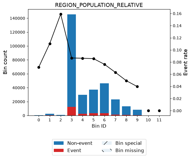
binning_table.plot(metric="event_rate")