Tutorial: optimal binning with continuous target
Basic
To get us started, let’s load a well-known dataset from the UCI repository and transform the data into a pandas.DataFrame.
[1]:
import matplotlib.pyplot as plt
import numpy as np
import pandas as pd
[2]:
class Data:
    def __init__(self, data, target, feature_names):
        self.data = data
        self.target = target
        self.feature_names = feature_names


def load_boston():
    data_url = "../../../tests/data/boston_housing.csv"
    raw_df = pd.read_csv(data_url, sep=r"\s+", skiprows=22, header=None)
    raw_data = np.hstack([raw_df.values[::2, :], raw_df.values[1::2, :2]])
    target = raw_df.values[1::2, 2]
    feature_names = ['CRIM', 'ZN', 'INDUS', 'CHAS', 'NOX', 'RM', 'AGE', 'DIS',
                     'RAD', 'TAX', 'PTRATIO', 'B', 'LSTAT']

    return Data(raw_data, target, feature_names)

data = load_boston()
df = pd.DataFrame(data.data, columns=data.feature_names)
We choose a variable to discretize and the continuous target.
[3]:
variable = "LSTAT"
x = df[variable].values
y = data.target
Import and instantiate an ContinuousOptimalBinning object class. We pass the variable name and its data type.
[4]:
from optbinning import ContinuousOptimalBinning
[5]:
optb = ContinuousOptimalBinning(name=variable, dtype="numerical")
We fit the optimal binning object with arrays x and y.
[6]:
optb.fit(x, y)
[6]:
ContinuousOptimalBinning(name='LSTAT')In a Jupyter environment, please rerun this cell to show the HTML representation or trust the notebook.
On GitHub, the HTML representation is unable to render, please try loading this page with nbviewer.org.
Parameters
| name | 'LSTAT' | |
| dtype | 'numerical' | |
| prebinning_method | 'cart' | |
| max_n_prebins | 20 | |
| min_prebin_size | 0.05 | |
| min_n_bins | None | |
| max_n_bins | None | |
| min_bin_size | None | |
| max_bin_size | None | |
| monotonic_trend | 'auto' | |
| min_mean_diff | 0 | |
| max_pvalue | None | |
| max_pvalue_policy | 'consecutive' | |
| gamma | 0 | |
| outlier_detector | None | |
| outlier_params | None | |
| cat_cutoff | None | |
| cat_unknown | None | |
| user_splits | None | |
| user_splits_fixed | None | |
| special_codes | None | |
| split_digits | None | |
| time_limit | 100 | |
| verbose | False |
You can check if an optimal solution has been found via the status attribute:
[7]:
optb.status
[7]:
'OPTIMAL'
You can also retrieve the optimal split points via the splits attribute:
[8]:
optb.splits
[8]:
array([ 4.6500001 ,  5.49499989,  6.86500001,  9.7249999 , 13.0999999 ,
       14.4000001 , 17.23999977, 19.89999962, 23.31500053])
The binning table
The optimal binning algorithms return a binning table; a binning table displays the binned data and several metrics for each bin. Class ContinuousOptimalBinning returns an object ContinuousBinningTable via the binning_table attribute.
[9]:
binning_table = optb.binning_table
[10]:
type(binning_table)
[10]:
optbinning.binning.binning_statistics.ContinuousBinningTable
The binning_table is instantiated, but not built. Therefore, the first step is to call the method build, which returns a pandas.DataFrame.
[11]:
binning_table.build()
[11]:
| Bin | Count | Count (%) | Sum | Std | Mean | Min | Max | Zeros count | WoE | IV | |
|---|---|---|---|---|---|---|---|---|---|---|---|
| 0 | (-inf, 4.65) | 50 | 0.098814 | 1985.9 | 8.198651 | 39.718000 | 22.8 | 50.0 | 0 | 17.185194 | 1.698142 |
| 1 | [4.65, 5.49) | 28 | 0.055336 | 853.2 | 6.123541 | 30.471429 | 21.9 | 50.0 | 0 | 7.938622 | 0.439291 |
| 2 | [5.49, 6.87) | 45 | 0.088933 | 1188.6 | 5.136259 | 26.413333 | 20.6 | 48.8 | 0 | 3.880527 | 0.345106 |
| 3 | [6.87, 9.72) | 89 | 0.175889 | 2274.9 | 6.84525 | 25.560674 | 11.9 | 50.0 | 0 | 3.027868 | 0.532570 |
| 4 | [9.72, 13.10) | 84 | 0.166008 | 1755.4 | 2.949979 | 20.897619 | 14.5 | 31.0 | 0 | -1.635187 | 0.271454 |
| 5 | [13.10, 14.40) | 32 | 0.063241 | 667.4 | 2.632482 | 20.856250 | 15.0 | 29.6 | 0 | -1.676556 | 0.106027 |
| 6 | [14.40, 17.24) | 60 | 0.118577 | 1037.5 | 3.588003 | 17.291667 | 10.2 | 30.7 | 0 | -5.241140 | 0.621479 |
| 7 | [17.24, 19.90) | 43 | 0.084980 | 714.3 | 4.032554 | 16.611628 | 8.3 | 27.5 | 0 | -5.921178 | 0.503183 |
| 8 | [19.90, 23.32) | 28 | 0.055336 | 368.4 | 3.912839 | 13.157143 | 5.0 | 21.7 | 0 | -9.375663 | 0.518811 |
| 9 | [23.32, inf) | 47 | 0.092885 | 556.0 | 4.006586 | 11.829787 | 5.0 | 23.7 | 0 | -10.703019 | 0.994154 |
| 10 | Special | 0 | 0.000000 | 0.0 | NaN | 0.000000 | NaN | NaN | 0 | -22.532806 | 0.000000 |
| 11 | Missing | 0 | 0.000000 | 0.0 | NaN | 0.000000 | NaN | NaN | 0 | -22.532806 | 0.000000 |
| Totals | 506 | 1.000000 | 11401.6 | 22.532806 | 5.0 | 50.0 | 0 | 111.650568 | 6.030218 |
Let’s describe the columns of this binning table:
Bin: the intervals delimited by the optimal split points.
Count: the number of records for each bin.
Count (%): the percentage of records for each bin.
Sum: the target sum for each bin.
Std: the target std for each bin.
Mean: the target mean for each bin.
Min: the target min value for each bin.
Max: the target max value for each bin.
Zeros count: the number of zeros for each bin.
WoE: Surrogate Weight-of-Evidence for each bin.
IV: Surrogate IV for each bin.
The WoE IV for a continuous target is computed as follows:
\begin{equation} IV = \sum_{i=1}^n \text{WoE}_i \frac{r_i}{r_T}, \quad \text{WoE}_i = |U_i - \mu|, \end{equation}
where \(U_i\) is the target mean value for each bin, \(\mu\) is the total target mean, \(r_i\) is the number of records for each bin, and \(r_T\) is the total number of records.
The last row shows the total number of records, sum and mean.
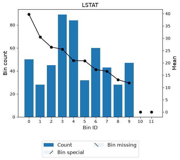
You can use the method plot to visualize the histogram and mean curve. Note that the Bin ID corresponds to the binning table index.
[12]:
binning_table.plot()
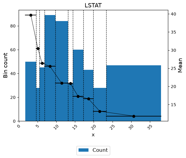
Optionally, you can show the binning plot with the actual bin widths.
[13]:
binning_table.plot(style="actual")
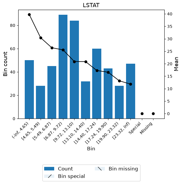
Or show the bin labels instead of bin ids.
[14]:
binning_table.plot(show_bin_labels=True)
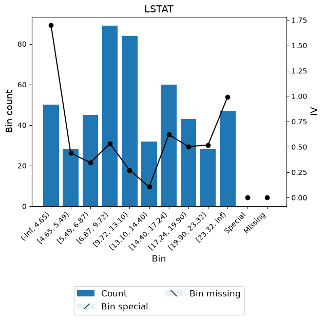
From version 0.19.0 the parameter metric is exposed to visualize other IV and WOE
[15]:
binning_table.plot(metric='iv', show_bin_labels=True)
Mean transformation
Now that we have checked the binned data, we can transform our original data into mean values. You can check the correctness of the transformation using pandas value_counts method, for instance.
[16]:
x_transform_bins = optb.transform(x, metric="bins")
[17]:
pd.Series(x_transform_bins).value_counts()
[17]:
[6.87, 9.72)      89
[9.72, 13.10)     84
[14.40, 17.24)    60
(-inf, 4.65)      50
[23.32, inf)      47
[5.49, 6.87)      45
[17.24, 19.90)    43
[13.10, 14.40)    32
[4.65, 5.49)      28
[19.90, 23.32)    28
Name: count, dtype: int64
Advanced
Many of the advanced options have been covered in the previous tutorials with a binary target. Check it out! In this section, we focus on the mean monotonicity trend and the mean difference between bins.
Binning table statistical analysis
The analysis method performs a statistical analysis of the binning table, computing the Information Value (IV), Weight of Evidence (WoE), and Herfindahl-Hirschman Index (HHI). Additionally, several statistical significance tests between consecutive bins of the contingency table are performed using the Student’s t-test.
[18]:
binning_table.analysis()
-------------------------------------------------
OptimalBinning: Continuous Binning Table Analysis
-------------------------------------------------

  General metrics

    IV                       6.03021763
    WoE                    111.65056765
    WoE (normalized)         4.95502274
    HHI                      0.11620241
    HHI (normalized)         0.01800268
    Quality score            0.01358682

  Monotonic trend            descending

  Significance tests

    Bin A  Bin B  t-statistic      p-value
        0      1     5.644492 3.313748e-07
        1      2     2.924528 5.175586e-03
        2      3     0.808313 4.206096e-01
        3      4     5.874488 3.816654e-08
        4      5     0.073112 9.419504e-01
        5      6     5.428848 5.770714e-07
        6      7     0.883289 3.796030e-01
        7      8     3.591859 6.692488e-04
        8      9     1.408305 1.643801e-01
Mean monotonicity
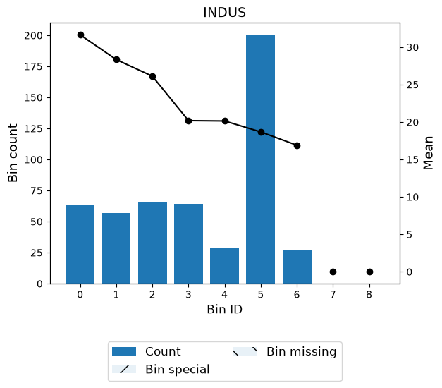
The monotonic_trend option permits forcing a monotonic trend to the mean curve. The default setting “auto” should be the preferred option, however, some business constraints might require to impose different trends. The default setting “auto” chooses the monotonic trend most likely to minimize the L1-norm from the options “ascending”, “descending”, “peak” and “valley” using a machine-learning-based classifier.
[19]:
variable = "INDUS"
x = df[variable].values
[20]:
optb = ContinuousOptimalBinning(name=variable, dtype="numerical",
                                monotonic_trend="auto")
optb.fit(x, y)
[20]:
ContinuousOptimalBinning(name='INDUS')In a Jupyter environment, please rerun this cell to show the HTML representation or trust the notebook.
On GitHub, the HTML representation is unable to render, please try loading this page with nbviewer.org.
Parameters
| name | 'INDUS' | |
| dtype | 'numerical' | |
| prebinning_method | 'cart' | |
| max_n_prebins | 20 | |
| min_prebin_size | 0.05 | |
| min_n_bins | None | |
| max_n_bins | None | |
| min_bin_size | None | |
| max_bin_size | None | |
| monotonic_trend | 'auto' | |
| min_mean_diff | 0 | |
| max_pvalue | None | |
| max_pvalue_policy | 'consecutive' | |
| gamma | 0 | |
| outlier_detector | None | |
| outlier_params | None | |
| cat_cutoff | None | |
| cat_unknown | None | |
| user_splits | None | |
| user_splits_fixed | None | |
| special_codes | None | |
| split_digits | None | |
| time_limit | 100 | |
| verbose | False |
[21]:
binning_table = optb.binning_table
binning_table.build()
[21]:
| Bin | Count | Count (%) | Sum | Std | Mean | Min | Max | Zeros count | WoE | IV | |
|---|---|---|---|---|---|---|---|---|---|---|---|
| 0 | (-inf, 3.35) | 63 | 0.124506 | 1994.0 | 8.569841 | 31.650794 | 16.5 | 50.0 | 0 | 9.117987 | 1.135243 |
| 1 | [3.35, 5.04) | 57 | 0.112648 | 1615.2 | 8.07271 | 28.336842 | 17.2 | 50.0 | 0 | 5.804036 | 0.653814 |
| 2 | [5.04, 6.66) | 66 | 0.130435 | 1723.7 | 7.879078 | 26.116667 | 16.0 | 50.0 | 0 | 3.583860 | 0.467460 |
| 3 | [6.66, 9.12) | 64 | 0.126482 | 1292.0 | 4.614126 | 20.187500 | 12.7 | 35.2 | 0 | -2.345306 | 0.296640 |
| 4 | [9.12, 10.30) | 29 | 0.057312 | 584.1 | 2.252281 | 20.141379 | 16.1 | 24.5 | 0 | -2.391427 | 0.137058 |
| 5 | [10.30, 20.73) | 200 | 0.395257 | 3736.2 | 8.959305 | 18.681000 | 5.0 | 50.0 | 0 | -3.851806 | 1.522453 |
| 6 | [20.73, inf) | 27 | 0.053360 | 456.4 | 3.690878 | 16.903704 | 7.0 | 23.0 | 0 | -5.629103 | 0.300367 |
| 7 | Special | 0 | 0.000000 | 0.0 | NaN | 0.000000 | NaN | NaN | 0 | -22.532806 | 0.000000 |
| 8 | Missing | 0 | 0.000000 | 0.0 | NaN | 0.000000 | NaN | NaN | 0 | -22.532806 | 0.000000 |
| Totals | 506 | 1.000000 | 11401.6 | 22.532806 | 5.0 | 50.0 | 0 | 77.789138 | 4.513036 |
[22]:
binning_table.plot()
[23]:
optb.information()
optbinning (Version 1.0.0)
Copyright (c) 2019-2026 Guillermo Navas-Palencia, Apache License 2.0

  Name    : INDUS
  Status  : OPTIMAL

  Pre-binning statistics
    Number of pre-bins                    13
    Number of refinements                  0

  Solver statistics
    Type                                  cp
    Number of booleans                    95
    Number of branches                   500
    Number of conflicts                   17
    Objective value                 32723523
    Best objective bound            32723523

  Timing
    Total time                          0.14 sec
    Pre-processing                      0.00 sec   (  1.37%)
    Pre-binning                         0.01 sec   (  5.49%)
    Solver                              0.13 sec   ( 92.67%)
      model generation                  0.05 sec   ( 37.87%)
      optimizer                         0.08 sec   ( 62.13%)
    Post-processing                     0.00 sec   (  0.19%)
[24]:
binning_table.analysis()
-------------------------------------------------
OptimalBinning: Continuous Binning Table Analysis
-------------------------------------------------

  General metrics

    IV                       4.51303567
    WoE                     77.78913838
    WoE (normalized)         3.45226144
    HHI                      0.22356231
    HHI (normalized)         0.09415603
    Quality score            0.02471482

  Monotonic trend            descending

  Significance tests

    Bin A  Bin B  t-statistic      p-value
        0      1     2.180865 3.118080e-02
        1      2     1.537968 1.267445e-01
        2      3     5.254539 7.781110e-07
        3      4     0.064736 9.485275e-01
        4      5     1.923770 5.601023e-02
        5      6     1.867339 6.563949e-02
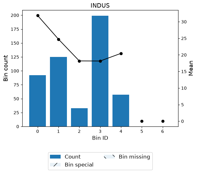
A smoother curve, keeping the valley monotonicity, can be achieved by using monotonic_trend="convex".
[25]:
optb = ContinuousOptimalBinning(name=variable, dtype="numerical",
                                monotonic_trend="convex")
optb.fit(x, y)
[25]:
ContinuousOptimalBinning(monotonic_trend='convex', name='INDUS')In a Jupyter environment, please rerun this cell to show the HTML representation or trust the notebook.
On GitHub, the HTML representation is unable to render, please try loading this page with nbviewer.org.
Parameters
| name | 'INDUS' | |
| monotonic_trend | 'convex' | |
| dtype | 'numerical' | |
| prebinning_method | 'cart' | |
| max_n_prebins | 20 | |
| min_prebin_size | 0.05 | |
| min_n_bins | None | |
| max_n_bins | None | |
| min_bin_size | None | |
| max_bin_size | None | |
| min_mean_diff | 0 | |
| max_pvalue | None | |
| max_pvalue_policy | 'consecutive' | |
| gamma | 0 | |
| outlier_detector | None | |
| outlier_params | None | |
| cat_cutoff | None | |
| cat_unknown | None | |
| user_splits | None | |
| user_splits_fixed | None | |
| special_codes | None | |
| split_digits | None | |
| time_limit | 100 | |
| verbose | False |
[26]:
binning_table = optb.binning_table
binning_table.build()
[26]:
| Bin | Count | Count (%) | Sum | Std | Mean | Min | Max | Zeros count | WoE | IV | |
|---|---|---|---|---|---|---|---|---|---|---|---|
| 0 | (-inf, 3.99) | 92 | 0.181818 | 2932.6 | 8.688703 | 31.876087 | 16.5 | 50.0 | 0 | 9.343281 | 1.698778 |
| 1 | [3.99, 8.01) | 125 | 0.247036 | 3092.3 | 6.644213 | 24.738400 | 14.4 | 50.0 | 0 | 2.205594 | 0.544860 |
| 2 | [8.01, 9.12) | 33 | 0.065217 | 600.0 | 3.614571 | 18.181818 | 12.7 | 27.5 | 0 | -4.350988 | 0.283760 |
| 3 | [9.12, 18.84) | 199 | 0.393281 | 3610.8 | 7.540328 | 18.144724 | 5.0 | 50.0 | 0 | -4.388083 | 1.725748 |
| 4 | [18.84, inf) | 57 | 0.112648 | 1165.9 | 9.519086 | 20.454386 | 7.0 | 50.0 | 0 | -2.078420 | 0.234130 |
| 5 | Special | 0 | 0.000000 | 0.0 | NaN | 0.000000 | NaN | NaN | 0 | -22.532806 | 0.000000 |
| 6 | Missing | 0 | 0.000000 | 0.0 | NaN | 0.000000 | NaN | NaN | 0 | -22.532806 | 0.000000 |
| Totals | 506 | 1.000000 | 11401.6 | 22.532806 | 5.0 | 50.0 | 0 | 67.431978 | 4.487277 |
[27]:
binning_table.plot()
[28]:
binning_table.analysis()
-------------------------------------------------
OptimalBinning: Continuous Binning Table Analysis
-------------------------------------------------

  General metrics

    IV                       4.48727679
    WoE                     67.43197816
    WoE (normalized)         2.99261340
    HHI                      0.26569701
    HHI (normalized)         0.08212126
    Quality score            0.01974910

  Monotonic trend       valley (convex)

  Significance tests

    Bin A  Bin B  t-statistic      p-value
        0      1     6.588254 5.789868e-10
        1      2     7.575550 2.331580e-11
        2      3     0.044930 9.642654e-01
        3      4    -1.686553 9.572501e-02
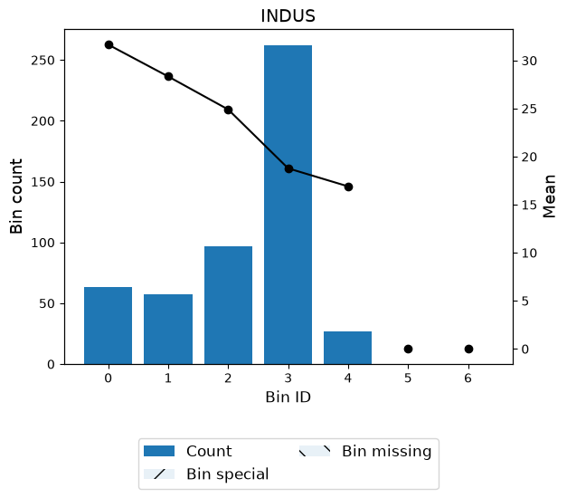
For example, we can force the variable INDUS (proportion of non-retail business acres per town) to be monotonically descending with respect to the house-pric and satisfy a max p-value constraint.
[29]:
optb = ContinuousOptimalBinning(name=variable, dtype="numerical",
                                monotonic_trend="descending",
                                max_pvalue=0.05)
optb.fit(x, y)
[29]:
ContinuousOptimalBinning(max_pvalue=0.05, monotonic_trend='descending',
                         name='INDUS')
In a Jupyter environment, please rerun this cell to show the HTML representation or trust the notebook. On GitHub, the HTML representation is unable to render, please try loading this page with nbviewer.org.
Parameters
| name | 'INDUS' | |
| monotonic_trend | 'descending' | |
| max_pvalue | 0.05 | |
| dtype | 'numerical' | |
| prebinning_method | 'cart' | |
| max_n_prebins | 20 | |
| min_prebin_size | 0.05 | |
| min_n_bins | None | |
| max_n_bins | None | |
| min_bin_size | None | |
| max_bin_size | None | |
| min_mean_diff | 0 | |
| max_pvalue_policy | 'consecutive' | |
| gamma | 0 | |
| outlier_detector | None | |
| outlier_params | None | |
| cat_cutoff | None | |
| cat_unknown | None | |
| user_splits | None | |
| user_splits_fixed | None | |
| special_codes | None | |
| split_digits | None | |
| time_limit | 100 | |
| verbose | False |
[30]:
binning_table = optb.binning_table
binning_table.build()
[30]:
| Bin | Count | Count (%) | Sum | Std | Mean | Min | Max | Zeros count | WoE | IV | |
|---|---|---|---|---|---|---|---|---|---|---|---|
| 0 | (-inf, 3.35) | 63 | 0.124506 | 1994.0 | 8.569841 | 31.650794 | 16.5 | 50.0 | 0 | 9.117987 | 1.135243 |
| 1 | [3.35, 5.04) | 57 | 0.112648 | 1615.2 | 8.07271 | 28.336842 | 17.2 | 50.0 | 0 | 5.804036 | 0.653814 |
| 2 | [5.04, 8.01) | 97 | 0.191700 | 2415.7 | 7.221288 | 24.904124 | 14.4 | 50.0 | 0 | 2.371317 | 0.454581 |
| 3 | [8.01, 20.73) | 262 | 0.517787 | 4920.3 | 7.983667 | 18.779771 | 5.0 | 50.0 | 0 | -3.753035 | 1.943271 |
| 4 | [20.73, inf) | 27 | 0.053360 | 456.4 | 3.690878 | 16.903704 | 7.0 | 23.0 | 0 | -5.629103 | 0.300367 |
| 5 | Special | 0 | 0.000000 | 0.0 | NaN | 0.000000 | NaN | NaN | 0 | -22.532806 | 0.000000 |
| 6 | Missing | 0 | 0.000000 | 0.0 | NaN | 0.000000 | NaN | NaN | 0 | -22.532806 | 0.000000 |
| Totals | 506 | 1.000000 | 11401.6 | 22.532806 | 5.0 | 50.0 | 0 | 71.741091 | 4.487277 |
[31]:
binning_table.plot()
[32]:
binning_table.analysis()
-------------------------------------------------
OptimalBinning: Continuous Binning Table Analysis
-------------------------------------------------

  General metrics

    IV                       4.48727679
    WoE                     71.74109110
    WoE (normalized)         3.18385070
    HHI                      0.33589027
    HHI (normalized)         0.16986283
    Quality score            0.52774693

  Monotonic trend            descending

  Significance tests

    Bin A  Bin B  t-statistic      p-value
        0      1     2.180865 3.118080e-02
        1      2     2.647685 9.326789e-03
        2      3     6.930572 6.470796e-11
        3      4     2.169454 3.432174e-02
Mininum mean difference between consecutive bins
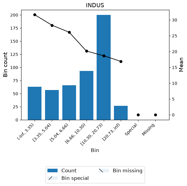
Now, we note that the mean difference between consecutive bins is not significant enough. Therefore, we decide to set min_mean_diff=1.0:
[33]:
optb = ContinuousOptimalBinning(name=variable, dtype="numerical",
                                monotonic_trend="descending", min_mean_diff=1.0)
optb.fit(x, y)
[33]:
ContinuousOptimalBinning(min_mean_diff=1.0, monotonic_trend='descending',
                         name='INDUS')
In a Jupyter environment, please rerun this cell to show the HTML representation or trust the notebook. On GitHub, the HTML representation is unable to render, please try loading this page with nbviewer.org.
Parameters
| name | 'INDUS' | |
| monotonic_trend | 'descending' | |
| min_mean_diff | 1.0 | |
| dtype | 'numerical' | |
| prebinning_method | 'cart' | |
| max_n_prebins | 20 | |
| min_prebin_size | 0.05 | |
| min_n_bins | None | |
| max_n_bins | None | |
| min_bin_size | None | |
| max_bin_size | None | |
| max_pvalue | None | |
| max_pvalue_policy | 'consecutive' | |
| gamma | 0 | |
| outlier_detector | None | |
| outlier_params | None | |
| cat_cutoff | None | |
| cat_unknown | None | |
| user_splits | None | |
| user_splits_fixed | None | |
| special_codes | None | |
| split_digits | None | |
| time_limit | 100 | |
| verbose | False |
[34]:
binning_table = optb.binning_table
binning_table.build()
[34]:
| Bin | Count | Count (%) | Sum | Std | Mean | Min | Max | Zeros count | WoE | IV | |
|---|---|---|---|---|---|---|---|---|---|---|---|
| 0 | (-inf, 3.35) | 63 | 0.124506 | 1994.0 | 8.569841 | 31.650794 | 16.5 | 50.0 | 0 | 9.117987 | 1.135243 |
| 1 | [3.35, 5.04) | 57 | 0.112648 | 1615.2 | 8.07271 | 28.336842 | 17.2 | 50.0 | 0 | 5.804036 | 0.653814 |
| 2 | [5.04, 6.66) | 66 | 0.130435 | 1723.7 | 7.879078 | 26.116667 | 16.0 | 50.0 | 0 | 3.583860 | 0.467460 |
| 3 | [6.66, 10.30) | 93 | 0.183794 | 1876.1 | 4.029092 | 20.173118 | 12.7 | 35.2 | 0 | -2.359688 | 0.433698 |
| 4 | [10.30, 20.73) | 200 | 0.395257 | 3736.2 | 8.959305 | 18.681000 | 5.0 | 50.0 | 0 | -3.851806 | 1.522453 |
| 5 | [20.73, inf) | 27 | 0.053360 | 456.4 | 3.690878 | 16.903704 | 7.0 | 23.0 | 0 | -5.629103 | 0.300367 |
| 6 | Special | 0 | 0.000000 | 0.0 | NaN | 0.000000 | NaN | NaN | 0 | -22.532806 | 0.000000 |
| 7 | Missing | 0 | 0.000000 | 0.0 | NaN | 0.000000 | NaN | NaN | 0 | -22.532806 | 0.000000 |
| Totals | 506 | 1.000000 | 11401.6 | 22.532806 | 5.0 | 50.0 | 0 | 75.412093 | 4.513036 |
[35]:
binning_table.plot(show_bin_labels=True)
[36]:
binning_table.analysis()
-------------------------------------------------
OptimalBinning: Continuous Binning Table Analysis
-------------------------------------------------

  General metrics

    IV                       4.51303567
    WoE                     75.41209309
    WoE (normalized)         3.34676880
    HHI                      0.23806027
    HHI (normalized)         0.08567233
    Quality score            0.48135484

  Monotonic trend            descending

  Significance tests

    Bin A  Bin B  t-statistic      p-value
        0      1     2.180865 3.118080e-02
        1      2     1.537968 1.267445e-01
        2      3     5.628303 2.077284e-07
        3      4     1.966209 5.022562e-02
        4      5     1.867339 6.563949e-02
Handle outliers
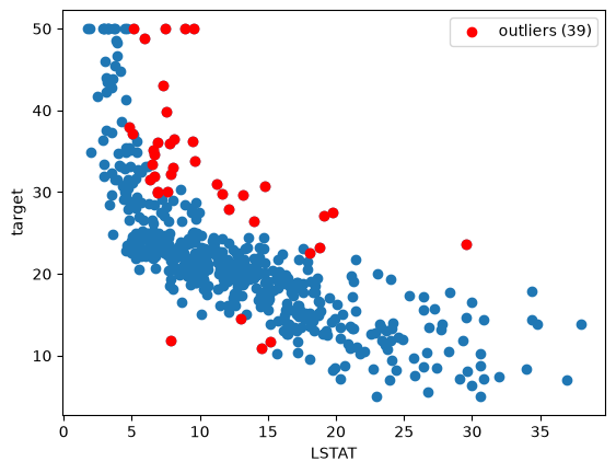
Version 0.16.1 introduced the outlier detector YQuantileDetector, specially designed to remove outliers for the ContinuousOptimalBinning algorithm. The application of this detector permits obtaining mean values per bin more similar to those obtained with more robust statistics (e.g., the median).
[37]:
from optbinning.binning.outlier import YQuantileDetector
[38]:
variable = "LSTAT"
x = df[variable].values
[39]:
detector = YQuantileDetector(n_bins=10, outlier_detector="range",
                             outlier_params={'method': 'HDI'})
detector.fit(x, y)
[39]:
YQuantileDetector(n_bins=10, outlier_detector='range',
                  outlier_params={'method': 'HDI'})
In a Jupyter environment, please rerun this cell to show the HTML representation or trust the notebook. On GitHub, the HTML representation is unable to render, please try loading this page with nbviewer.org.
Parameters
| outlier_detector | 'range' | |
| outlier_params | {'method': 'HDI'} | |
| n_bins | 10 |
[40]:
plt.scatter(x, y)

mask = detector.get_support()
plt.scatter(x[mask], y[mask], color='r', label=f"outliers ({np.count_nonzero(mask)})")

plt.xlabel(variable)
plt.ylabel("target")

plt.legend()
plt.show()
[41]:
optb = ContinuousOptimalBinning(name=variable, dtype="numerical",
                                monotonic_trend="descending",
                                outlier_detector="yquantile",
                                outlier_params={
                                    'n_bins': 10,
                                    'outlier_detector': 'range',
                                    'outlier_params': {'method': 'HDI'}
                                },
                               verbose=True)
optb.fit(x, y)
2026-09-12 18:06:17,363 | INFO : Optimal binning started.
2026-09-12 18:06:17,365 | INFO : Options: check parameters.
2026-09-12 18:06:17,368 | INFO : Pre-processing started.
2026-09-12 18:06:17,373 | INFO : Pre-processing: number of samples: 506
2026-09-12 18:06:17,387 | INFO : Pre-processing: number of clean samples: 467
2026-09-12 18:06:17,389 | INFO : Pre-processing: number of missing samples: 0
2026-09-12 18:06:17,391 | INFO : Pre-processing: number of special samples: 0
2026-09-12 18:06:17,392 | INFO : Pre-processing: number of outlier samples: 39
2026-09-12 18:06:17,394 | INFO : Pre-processing terminated. Time: 0.0119s
2026-09-12 18:06:17,395 | INFO : Pre-binning started.
2026-09-12 18:06:17,402 | INFO : Pre-binning: number of prebins: 14
2026-09-12 18:06:17,403 | INFO : Pre-binning terminated. Time: 0.0063s
2026-09-12 18:06:17,405 | INFO : Optimizer started.
2026-09-12 18:06:17,407 | INFO : Optimizer: monotonic trend set to descending.
2026-09-12 18:06:17,408 | INFO : Optimizer: build model...
2026-09-12 18:06:17,456 | INFO : Optimizer: solve...
2026-09-12 18:06:17,513 | INFO : Optimizer terminated. Time: 0.1058s
2026-09-12 18:06:17,515 | INFO : Post-processing started.
2026-09-12 18:06:17,516 | INFO : Post-processing: compute binning information.
2026-09-12 18:06:17,518 | INFO : Post-processing terminated. Time: 0.0003s
2026-09-12 18:06:17,520 | INFO : Optimal binning terminated. Status: OPTIMAL. Time: 0.1578s
[41]:
ContinuousOptimalBinning(monotonic_trend='descending', name='LSTAT',
                         outlier_detector='yquantile',
                         outlier_params={'n_bins': 10,
                                         'outlier_detector': 'range',
                                         'outlier_params': {'method': 'HDI'}},
                         verbose=True)
In a Jupyter environment, please rerun this cell to show the HTML representation or trust the notebook. On GitHub, the HTML representation is unable to render, please try loading this page with nbviewer.org.
Parameters
| name | 'LSTAT' | |
| monotonic_trend | 'descending' | |
| outlier_detector | 'yquantile' | |
| outlier_params | {'n_bins': 10, 'outlier_detector': 'range', 'outlier_params': {'method': 'HDI'}} | |
| verbose | True | |
| dtype | 'numerical' | |
| prebinning_method | 'cart' | |
| max_n_prebins | 20 | |
| min_prebin_size | 0.05 | |
| min_n_bins | None | |
| max_n_bins | None | |
| min_bin_size | None | |
| max_bin_size | None | |
| min_mean_diff | 0 | |
| max_pvalue | None | |
| max_pvalue_policy | 'consecutive' | |
| gamma | 0 | |
| cat_cutoff | None | |
| cat_unknown | None | |
| user_splits | None | |
| user_splits_fixed | None | |
| special_codes | None | |
| split_digits | None | |
| time_limit | 100 |
[42]:
optb.binning_table.build()
[42]:
| Bin | Count | Count (%) | Sum | Std | Mean | Min | Max | Zeros count | WoE | IV | |
|---|---|---|---|---|---|---|---|---|---|---|---|
| 0 | (-inf, 4.15) | 36 | 0.077088 | 1495.8 | 7.729866 | 41.550000 | 24.8 | 50.0 | 0 | 19.824732 | 1.528245 |
| 1 | [4.15, 5.49) | 39 | 0.083512 | 1218.2 | 6.428482 | 31.235897 | 21.9 | 50.0 | 0 | 9.510630 | 0.794250 |
| 2 | [5.49, 6.57) | 29 | 0.062099 | 735.1 | 3.174426 | 25.348276 | 20.6 | 33.2 | 0 | 3.623008 | 0.224983 |
| 3 | [6.57, 7.68) | 29 | 0.062099 | 705.8 | 2.035786 | 24.337931 | 20.7 | 29.1 | 0 | 2.612663 | 0.162242 |
| 4 | [7.68, 9.95) | 59 | 0.126338 | 1341.0 | 3.012688 | 22.728814 | 16.5 | 30.3 | 0 | 1.003546 | 0.126786 |
| 5 | [9.95, 11.67) | 42 | 0.089936 | 884.4 | 2.257068 | 21.057143 | 15.0 | 24.7 | 0 | -0.668125 | 0.060088 |
| 6 | [11.67, 13.74) | 49 | 0.104925 | 982.4 | 2.119503 | 20.048980 | 15.0 | 24.5 | 0 | -1.676288 | 0.175885 |
| 7 | [13.74, 15.00) | 28 | 0.059957 | 550.2 | 2.143012 | 19.650000 | 16.0 | 24.4 | 0 | -2.075268 | 0.124427 |
| 8 | [15.00, 17.11) | 37 | 0.079229 | 632.6 | 2.79483 | 17.097297 | 10.2 | 22.4 | 0 | -4.627970 | 0.366670 |
| 9 | [17.11, 18.93) | 38 | 0.081370 | 607.3 | 2.97081 | 15.981579 | 9.6 | 23.1 | 0 | -5.743689 | 0.467367 |
| 10 | [18.93, 21.95) | 26 | 0.055675 | 350.5 | 3.532271 | 13.480769 | 7.2 | 21.7 | 0 | -8.244498 | 0.459008 |
| 11 | [21.95, 26.44) | 27 | 0.057816 | 332.0 | 3.524148 | 12.296296 | 5.0 | 20.0 | 0 | -9.428971 | 0.545144 |
| 12 | [26.44, inf) | 28 | 0.059957 | 310.4 | 3.754589 | 11.085714 | 5.0 | 17.9 | 0 | -10.639553 | 0.637918 |
| 13 | Special | 0 | 0.000000 | 0.0 | NaN | 0.000000 | NaN | NaN | 0 | -21.725268 | 0.000000 |
| 14 | Missing | 0 | 0.000000 | 0.0 | NaN | 0.000000 | NaN | NaN | 0 | -21.725268 | 0.000000 |
| Totals | 467 | 1.000000 | 10145.7 | 21.725268 | 5.0 | 50.0 | 0 | 123.129478 | 5.673013 |
[43]:
optb.binning_table.plot()
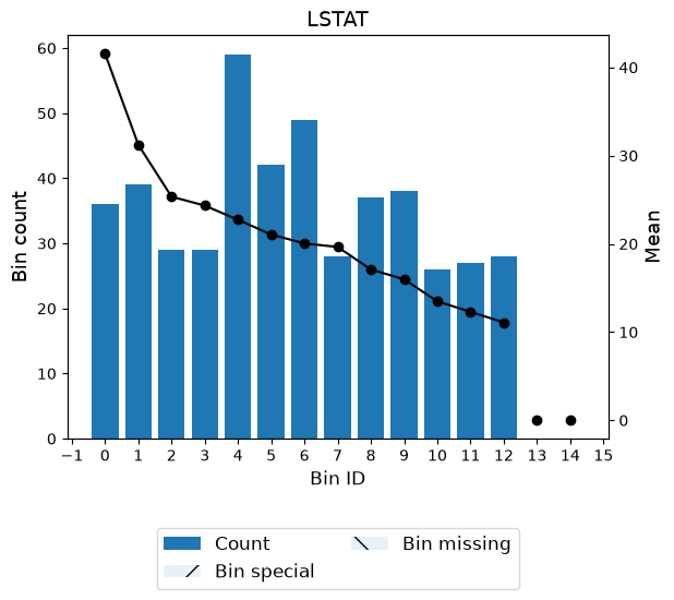
As observed in the logs, 39 outliers were removed during preprocessing. Compared to the standard binning, the resulting binning after removing outliers returns more bins (13 vs 10) and higher objective function (total WoE).
Sample weights
Finally, version 0.17.0 added support to sample weights. As an example, let’s increase the weights for values < 10.
[44]:
sample_weight = np.ones(len(x))
sample_weight[x < 10] = 5
[45]:
optb = ContinuousOptimalBinning(name=variable, dtype="numerical",
                                monotonic_trend="descending")
optb.fit(x, y, sample_weight=sample_weight)
[45]:
ContinuousOptimalBinning(monotonic_trend='descending', name='LSTAT')In a Jupyter environment, please rerun this cell to show the HTML representation or trust the notebook.
On GitHub, the HTML representation is unable to render, please try loading this page with nbviewer.org.
Parameters
| name | 'LSTAT' | |
| monotonic_trend | 'descending' | |
| dtype | 'numerical' | |
| prebinning_method | 'cart' | |
| max_n_prebins | 20 | |
| min_prebin_size | 0.05 | |
| min_n_bins | None | |
| max_n_bins | None | |
| min_bin_size | None | |
| max_bin_size | None | |
| min_mean_diff | 0 | |
| max_pvalue | None | |
| max_pvalue_policy | 'consecutive' | |
| gamma | 0 | |
| outlier_detector | None | |
| outlier_params | None | |
| cat_cutoff | None | |
| cat_unknown | None | |
| user_splits | None | |
| user_splits_fixed | None | |
| special_codes | None | |
| split_digits | None | |
| time_limit | 100 | |
| verbose | False |
[46]:
optb.binning_table.build()
[46]:
| Bin | Count | Count (%) | Sum | Std | Mean | Min | Max | Zeros count | WoE | IV | |
|---|---|---|---|---|---|---|---|---|---|---|---|
| 0 | (-inf, 3.32) | 90 | 0.065123 | 3959.0 | 6.404503 | 43.988889 | 160.0 | 250.0 | 0 | 17.056038 | 1.110741 |
| 1 | [3.32, 4.15) | 90 | 0.065123 | 3520.0 | 8.160126 | 39.111111 | 124.0 | 250.0 | 0 | 12.178260 | 0.793085 |
| 2 | [4.15, 4.65) | 70 | 0.050651 | 2450.5 | 7.456298 | 35.007143 | 114.0 | 250.0 | 0 | 8.074292 | 0.408973 |
| 3 | [4.65, 5.15) | 85 | 0.061505 | 2684.5 | 6.729237 | 31.582353 | 112.5 | 250.0 | 0 | 4.649502 | 0.285968 |
| 4 | [5.15, 5.94) | 120 | 0.086831 | 3337.0 | 6.024942 | 27.808333 | 103.0 | 244.0 | 0 | 0.875482 | 0.076019 |
| 5 | [5.94, 7.68) | 290 | 0.209841 | 7822.5 | 5.602603 | 26.974138 | 103.5 | 250.0 | 0 | 0.041287 | 0.008664 |
| 6 | [7.68, 8.13) | 80 | 0.057887 | 1965.0 | 6.760074 | 24.562500 | 59.5 | 182.5 | 0 | -2.370351 | 0.137213 |
| 7 | [8.13, 9.95) | 260 | 0.188133 | 6338.0 | 6.323023 | 24.376923 | 82.5 | 250.0 | 0 | -2.555928 | 0.480855 |
| 8 | [9.95, 12.47) | 71 | 0.051375 | 1488.7 | 2.797271 | 20.967606 | 15.0 | 101.5 | 0 | -5.965245 | 0.306463 |
| 9 | [12.47, 16.09) | 82 | 0.059334 | 1602.3 | 3.345651 | 19.540244 | 10.2 | 30.7 | 0 | -7.392607 | 0.438635 |
| 10 | [16.09, 20.19) | 71 | 0.051375 | 1154.1 | 3.675568 | 16.254930 | 8.3 | 27.5 | 0 | -10.677921 | 0.548576 |
| 11 | [20.19, inf) | 73 | 0.052822 | 899.6 | 4.026709 | 12.323288 | 5.0 | 23.7 | 0 | -14.609563 | 0.771706 |
| 12 | Special | 0 | 0.000000 | 0.0 | NaN | 0.000000 | NaN | NaN | 0 | -26.932851 | 0.000000 |
| 13 | Missing | 0 | 0.000000 | 0.0 | NaN | 0.000000 | NaN | NaN | 0 | -26.932851 | 0.000000 |
| Totals | 1382 | 1.000000 | 37221.2 | 26.932851 | 5.0 | 250.0 | 0 | 140.312179 | 5.366897 |
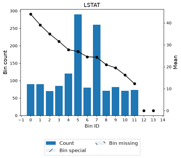
Note the count increase in the first bins.
[47]:
optb.binning_table.plot()